- Posted on
- admin
- No Comments
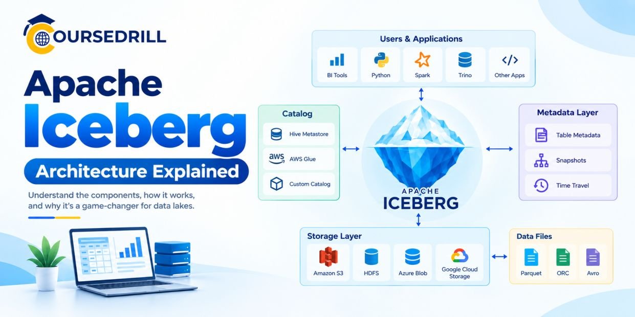
Apache Iceberg Architecture Explained
Creating a table, inserting some rows, and running a time-travel query gets you comfortable with Iceberg’s basic shape fast. What doesn’t show up in that first hour is the machinery that makes updates and deletes actually correct under concurrent writers, why an UPDATE on a billion-row table can complete in seconds instead of hours, or what genuinely changed when the spec moved from v1 to v2 to v3.
If you’re new to Iceberg entirely, our beginner’s tutorial covers the catalog, metadata file, manifest list, and manifest file hierarchy with a hands-on Trino quickstart. This piece assumes that foundation and goes further, into sequence numbers, row-level deletes, the three format versions, Puffin files, branches, and compaction, the parts of the spec that explain Iceberg’s actual behavior under real production write patterns.
Sequence Numbers: The Ordering Primitive Underneath Everything
Before covering deletes, one concept needs to be in place first, because almost nothing about correct delete handling makes sense without it. (cite index=”53-1″>Iceberg uses sequence numbers to track the order of changes made to the data. The sequence_number in a delete file indicates when the deletion was committed relative to other changes in the dataset.
(cite index=”51-1″>Each data file and delete file in Iceberg gets assigned a sequence number. When you delete a record, the delete file receives a higher sequence number than the existing data files it applies to. This ensures that newer records aren’t mistakenly deleted if they match the deletion criteria. Concretely: if a delete file says “remove rows where customer_id = 42” and was committed at sequence number 8, it only applies to data files with a sequence number less than 8. A data file written afterward, at sequence number 9, containing a legitimately new row with customer_id = 42, is untouched by that older delete, because the delete’s sequence number doesn’t cover it.
(cite index=”55-1″>The real Iceberg rules use field IDs, partitions, and sequence numbers together to determine which data files and rows a given delete actually applies to, preventing an old delete from incorrectly removing a newer row that happens to reuse the same key.
This is the mechanism that makes snapshot isolation actually hold up under concurrent writers touching overlapping data, not just a nice property claimed in the docs.
Row-Level Deletes: Copy-on-Write vs. Merge-on-Read
This is arguably the single most consequential architectural decision in any Iceberg deployment, and it’s a decision you make per table, not a fixed property of the format.
Copy-on-write (COW) is the more intuitive approach: when a row needs to be deleted or updated, Iceberg rewrites the entire data file that row lived in, minus that row, and commits a new snapshot pointing at the replacement file. It’s simple to reason about and produces fast reads, since there’s nothing extra for a query to reconcile at read time, but it makes every write, even one touching a single row, as expensive as rewriting the whole file that row belongs to.
Merge-on-read (MOR) takes the opposite tradeoff. (cite index=”48-1″>Instead of rewriting data files, the engine writes small delete files that record the deleted row positions or equality conditions, then commits a new snapshot that includes both the original data files and the new delete files. (cite index=”51-1″>This dramatically speeds up write operations, since you’re only writing the changes rather than rewriting entire files. The trade-off surfaces at read time: when a query reads a MOR table, the engine must merge data files with delete files, and this merge adds overhead to every read, overhead that grows as delete files accumulate.
Within merge-on-read, there are two distinct kinds of delete files, and they solve different problems:
Positional delete files (cite index=”53-1″>specify the exact position of a row within a specific data file that should be marked as deleted, based on the physical layout of the data. (cite index=”48-1″>They’re efficient to read, a reader just skips a known row offset, but slower to write, since the writer needs to know exactly where the target row physically sits.
Equality delete files (cite index=”53-1″>contain the values that identify which rows should be deleted, for instance a specific ID value that needs to be removed across multiple data files, rather than tracking physical position at all. (cite index=”48-1″>This is more flexible, since one equality delete can retroactively apply to any matching row regardless of which file it’s in, but more expensive to evaluate at read time, since a reader has to check every row’s values against the delete condition rather than jumping straight to a known offset. While positional deletes are efficient to read but slower to write, equality deletes are quicker to write but require more processing during reads.
A useful real-world data point on the actual performance gap merge-on-read is designed to close: (cite index=”51-1″>in one benchmark, a 5-million-row update completed on an Iceberg MOR table in just over 2 minutes, compared to nearly 12 minutes for the equivalent update on PostgreSQL, illustrating why streaming and CDC-heavy pipelines lean so heavily on merge-on-read despite its read-time cost.
That read-time cost isn’t meant to be permanent, though. (cite index=”51-1″>The key to maintaining good performance with merge-on-read tables lies in regular compaction, covered in detail further down, which periodically folds accumulated delete files back into clean data files.
Format Versions: What Actually Changed From v1 to v3
Iceberg’s table format has evolved through three major versions, and understanding what each one actually added clarifies a lot of the terminology you’ll run into across different engines and vendor docs.
(cite index=”57-1″>Format version 1 is append-only, with no support for row-level deletes at all. Format version 2 introduces merge-on-read with both position and equality deletes, the mechanism covered above. Format version 3 introduces deletion vectors stored as Puffin files, along with row lineage tracking and default values for new columns.
The v3 change to deletion vectors is worth understanding specifically, since it directly addresses one of merge-on-read’s real operational headaches. (cite index=”64-1″>Under v2, an accumulation of individual positional delete files effectively becomes a “small-delete-file swarm”, lots of tiny files that themselves need tracking and eventually compacting.
Deletion vectors, compact bitmaps stored in Puffin files, replace that swarm of positional delete files with a single, denser structure per data file, giving O(1) per-file delete lookup via one bitmap instead of scanning a scattered set of small delete files. (cite index=”56-1″>The vector itself is a serialized bitmap where a set bit at a given position indicates the row at that position is deleted, using a collection of 32-bit Roaring bitmaps under the hood, optimized for the common case where most row positions fit comfortably in 32 bits.
(cite index=”64-1″>Equality deletes remain available in v3 for key-based CDC-style deletes where you don’t know a row’s physical position, but the positional-delete-file swarm specifically is gone, replaced by deletion vectors. It’s worth noting real-world adoption of v3 is still catching up across the ecosystem, some managed platforms currently support reading v3 tables but not yet writing them, so it’s worth checking your specific engine’s current v3 support before committing production write paths to it.
Puffin Files: The Sidecar Format for Statistics and Deletion Vectors
Puffin is worth understanding as its own concept, since it now serves two distinct purposes in the spec, not just deletion vectors.
(cite index=”63-1″>Table statistics files are themselves valid Puffin files. Statistics are informational, a reader can choose to ignore them entirely, since statistics support isn’t required to read a table correctly, but a table can accumulate many statistics files associated with different snapshots over its lifetime.
One specific statistic worth knowing about: (cite index=”56-1″>a Puffin blob can hold a serialized “compact” Theta sketch produced by the Apache DataSketches library, letting a query engine derive an estimate of the number of distinct values, an NDV estimate, for a column without scanning the full dataset. That’s a meaningful input for a cost-based optimizer trying to decide join order or estimate result cardinality, information a manifest file’s simple min/max bounds can’t provide on its own.
Partition Spec Evolution and Sort Orders
Just as schemas carry a version ID, so do partition specs, letting a table’s physical partitioning strategy change over time without a disruptive rewrite of historical data. Every data file’s manifest entry records which partition spec ID it was written under, and the query engine reads that mapping to interpret older files correctly even after the partitioning strategy has since changed. A table that started partitioned by day and later moved to monthly partitions doesn’t need its years of daily-partitioned history rewritten, both partition specs simply coexist in the table’s metadata, tagged by ID, and each file gets read according to whichever spec was active when it was written.
Sort orders work on the same versioned-ID principle. A table can declare that data should be physically sorted by a given set of columns on write, which, combined with compaction, is what actually determines how effectively file-level pruning statistics can eliminate files during query planning, covered next.
Branches and Tags: Git-Like Versioning for Tables
Beyond the default main branch every table implicitly has, Iceberg supports creating named branches and tags directly on a table, each with its own independent snapshot history and its own retention rules. Tags are typically used to pin an immutable, named reference to a specific snapshot indefinitely, useful for compliance holds or reproducible reporting periods. Branches behave more like a working area: a separate line of commits that can diverge from main, be validated, and later be merged or fast-forwarded into it.
That branching capability is what makes a specific, widely used data-quality pattern possible without any additional tooling beyond what Iceberg already provides.
The Write-Audit-Publish (WAP) Pattern
(cite index=”66-1″>The Write-Audit-Publish pattern is a data quality workflow using Apache Iceberg branches to write new data to an isolated staging branch, validate it with automated data quality checks, then publish it to the main branch only if validation passes. Iceberg doesn’t enforce the pattern itself, orchestrating and executing it is the compute engine’s job, Spark currently has the most mature tooling for it, though Flink supports equivalent workflows for streaming scenarios.
(cite index=”70-1″>In a typical ETL pipeline without this pattern, data written directly to the production table is immediately visible to downstream consumers, so if that data has quality issues, duplicates, unexpected nulls, out-of-range values, the bad data is already visible before anyone gets a chance to validate it. WAP closes that gap structurally rather than through after-the-fact monitoring: (cite index=”71-1″>new data is written to an isolated staging branch first, invisible to production consumers, automated quality checks run against that staging branch, and only if all checks pass does the staging branch get fast-forwarded or merged into main, making the new data visible.
(cite index=”68-1″>Iceberg’s fast_forward procedure moves the current snapshot of one branch to the latest snapshot of another, main to the head of an audit branch, for instance, once validation succeeds. The publish_changes procedure similarly creates a new snapshot from an existing staged one without altering or removing the original, giving engines two related mechanisms depending on whether the workflow needs a clean fast-forward or a more general publish operation.
(cite index=”67-1″>Beyond the WAP pattern itself, Iceberg’s tagging API also enables pinning immutable snapshots for compliance purposes, and (cite index=”71-1″>while Iceberg’s own WAP model operates at the table level, with each table getting its own staging branch, Project Nessie extends the same underlying idea to catalog-level WAP, a single branch that spans every table in the catalog at once, enabling cross-table atomic staging and publishing for pipelines that need multiple related tables to update together atomically.
Compaction: Undoing the Cost of Small Files and Accumulated Deletes
Every architectural choice covered above, frequent small commits, merge-on-read deletes, streaming ingestion, tends to produce the same operational byproduct over time: lots of small files and, on MOR tables, an accumulating pile of delete files that every read has to reconcile against. Compaction is the maintenance operation that reverses that decay.
(cite index=”69-1″>The default rewrite strategy is binpack, which simply rewrites smaller files into files closer to a target size and reconciles any delete files along the way, with no additional optimization like sorting. This is the fastest compaction strategy, so if minimizing compaction runtime matters most, binpack is usually the right default.
For better query-time performance rather than the fastest possible compaction job, (cite index=”69-1″>using a sort-based rewrite strategy can maximize the benefit of compaction, and z-order sorting specifically helps when queries commonly filter across multiple dimensions at once rather than a single sort key.
(cite index=”73-1″>Sort-based compaction organizes files according to a user-defined column order, clustering similar values together so that queries filtering on those columns scan meaningfully fewer files, reducing both query latency and compute cost. Reported real-world gains from switching from binpack to sort or z-order compaction have reached three times faster query performance or more, depending on data layout and query patterns, though the exact improvement is highly workload-dependent.
(cite index=”69-1″>Compaction also directly benefits merge-on-read tables specifically: rewriting files reconciles any accumulated delete files in the process, which improves subsequent read times since queries no longer need to merge those delete files at read time at all, they’re simply gone, folded into the newly compacted data files.
How This All Fits Into a Real Table Lifecycle
Tracing a realistic sequence of operations through everything above makes the architecture concrete. A streaming job appends new rows continuously, each micro-batch committing a new snapshot with its own sequence number. An hourly job runs UPDATE statements against yesterday’s data using merge-on-read, writing small delete files, positional if it knows exact row locations, equality if it’s identifying rows by a business key, each stamped with a sequence number higher than the data files it affects.
A nightly ETL pipeline uses the Write-Audit-Publish pattern, staging its output on a branch, running data-quality checks, and fast-forwarding into main only once those checks pass. Periodically, a scheduled maintenance job runs sort-based compaction against the most frequently queried partitions, reconciling accumulated delete files and clustering data for better pruning, while a separate job expires snapshots and orphaned files older than a defined retention window to keep metadata from growing unbounded.
None of these processes need to coordinate directly with each other beyond Iceberg’s own atomic catalog commits, and a query running mid-way through any of this still sees one single, fully consistent snapshot, never a partial view of an in-flight write.
Frequently Asked Questions
What’s the actual difference between copy-on-write and merge-on-read? Copy-on-write rewrites the entire data file a changed row belongs to, producing fast reads at the cost of expensive writes. Merge-on-read writes small delete files alongside the existing data instead, making writes much cheaper but requiring every subsequent read to reconcile those delete files against the underlying data until compaction cleans them up.
What’s the difference between positional and equality delete files? A positional delete file records the exact file and row offset to remove, which is fast for a reader to apply but requires the writer to know precisely where the target row lives. An equality delete file instead records a condition, like a specific ID value, that identifies rows to remove wherever they appear, which is cheaper to write but more expensive for a reader to evaluate against every row.
Why do sequence numbers matter for correctness? Sequence numbers establish a strict order between when data files and delete files were committed. A delete file only applies to data files with a lower sequence number than itself, which prevents a delete from incorrectly removing a legitimately new row that happens to share the same key as something deleted earlier.
What’s new in Iceberg v3 specifically? Iceberg v3 introduces deletion vectors, compact Roaring-bitmap-based structures stored in Puffin files that replace the accumulation of many small positional delete files, along with row lineage tracking and new data types including variant, geometry, and nanosecond-precision timestamps.
What is a Puffin file used for? Puffin is a sidecar file format used for two purposes in current versions of the spec: storing optional table statistics, like distinct-value estimates derived from Theta sketches, and, starting in v3, storing deletion vectors that mark deleted row positions as compact bitmaps.
What is the Write-Audit-Publish pattern and why use it? WAP uses Iceberg’s branching capability to stage new data on an isolated branch, run automated data quality checks against it, and only make it visible in the main table once those checks pass. It closes the gap where data written directly to a production table is visible to consumers before anyone has had a chance to validate it.
Which compaction strategy should I use? Binpack is the default and fastest option, rewriting small files toward a target size and reconciling delete files with no additional sorting. Sort-based or z-order compaction takes longer to run but can meaningfully improve query performance by clustering similar column values together, particularly worthwhile for tables with well-understood, frequently filtered query patterns.
Do I need to choose copy-on-write or merge-on-read for the whole table forever? No, it’s a table-level (and in some engines, operation-level) setting that can be changed, though switching modes doesn’t retroactively rewrite existing delete files or data files on its own. Some teams deliberately migrate a table from merge-on-read to copy-on-write specifically to simplify compatibility with engines that don’t yet support certain delete file types.
Final Thoughts
The features that make Iceberg feel almost magical in a beginner tutorial, instant schema changes, cheap deletes, reliable time travel, all trace back to the same small set of primitives covered here: sequence numbers establishing a strict order of truth, delete files (or, in v3, deletion vectors) recording changes without touching existing data, and an atomic catalog pointer ensuring every reader always sees one fully consistent state. Once those primitives are clear, decisions like choosing merge-on-read over copy-on-write, or picking a compaction strategy, stop being arbitrary configuration knobs and start looking like straightforward tradeoffs between write cost and read cost.
For the authoritative, versioned specification covering every detail referenced here, the Apache Iceberg table format spec is the definitive source, and it’s genuinely readable even for an engineer who isn’t building a table format implementation themselves. If you’re pairing Iceberg with Trino specifically, our Trino architecture guide covers how dynamic filtering and fault-tolerant execution interact directly with the manifest statistics and delete files described in this piece.
For more breakdowns of open-source data infrastructure and DevOps tooling like this one, keep exploring the guides on CourseDrill.
Popular Courses